June 8, 2010
This was a long run. Haviland started the data run at 3:55am GMT and stayed until 10:00am GMT, when Lauren took over until 2:20pm GMT, when it started raining. We wanted to observe the heating up of the boundary layer from pre-sunrise until sunset, but the rainy weather interfered. The sky was pretty clear at night, with no clouds visible but several stars out. Something was up at 14 km at 4:52am GMT that had been there a while. Nothing was visible on the skycam, but it was late at night, so something that high up might just not have enough light to be visible to the human eye. Other than the 14km spike, the night was very clear. Come morning, there were more clouds, especially at 12:22pm GMT when Lauren had to place the cloud cover over the primary mirror due to saturation. The cloud cover was taken off at 1:12pm GMT to check if the channels would still be saturated. Both the short and long range channels were fine, so the cloud cover stayed off. At 2:20pm GMT, Lauren had to close the hatch because it started to rain on the mirror, a few droplets. She waited thirty minutes for the rain to stop, but it never did, so she just shut down for the day. Overall, it was a clear night except the 14 km object, and it was a cloudy morning that eventually rained.
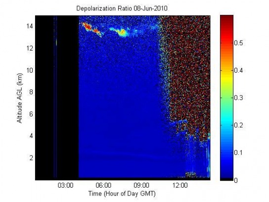
The 14km object can be seen in the Range Corrected Backscatter graph below, as well as the Depolarization Ratio graph. The Depolarization Ratio graph points out that the laser light being sent up is being depolarized, and is likely bouncing off of rough, jagged, or otherwise crystalline particles in the air. Usually, this indicates ice, aerosols, pollen, soot, etc. Due to the altitude and the shape, it is likely that the 14 km object is a cirrus cloud with high ice concentration. Above 7,000 m, ice freezes in the atmosphere due to the extremely cold temperatures. The object could also be a plane contrail, which are known to form into ice at high altitudes. The tropopause for this time was around 16 km, and planes generally fly either directly under or directly above the tropopause; so both cirrus clouds and plane contrails are a likely source for the depolarized backscatter.
Also, it is interesting to note that the little darker rectangle of blue on the colorized Range Corrected Backscatter graph happens during the same time that the cloud cover was on the primary mirror, from 12:22pm GMT until 1:12pm GMT. Therefore, it is probably safe to say that the cloud cover has an obvious effect on the graph of backscatter, as it should since it limits the amount of light that the mirror, and thus the digitizer, receives. Darker parts of future graphs that correlate with very small backscatter reception by EARL should be kept an eye on in lieu of the cloud mask effect. In the future, a correction can hopefully be made to the data with ProcEarl that accounts for a cloud mask being put on the primary mirror. However, the LIDAR equation must be first understood and solved, as well as a percentage of light blocked by the cloud cover be calculated.
The lack of data from 12:20am GMT until 3:55am GMT is due to a system check and EARL reallignment done before the attempted sunrise-sunset data run. It is interesting to note that, if more data had been taken from this point in time, the object at 14 km would likely still have been there; it can still be seen from the few minutes of data taken at about 1:00am GMT.
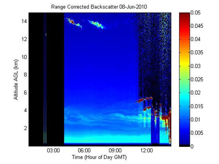
What on earth is the swirling waves of blue and turquoise indicating? This does not happen with most of the data sets. The turquoise got heavier and heavier in the section leading up to the rain. Perhaps this indicates an increase in humidity? What else could the swirling indicate? Turquoise suggests that the corresponding areas backscatter more light than the blue areas. But if this did not show up on the depolarization graph, then the swirling effect cannot be due to pollen or dust heating up and mixing about in the boundary layer. If the humidity was different at varying levels of the atmosphere, and if this humidity changed every few minutes at each varying level of the atmosphere, then that would explain the swirling effect. Humidity indicates an increase of water in the air, and more humidity in a certain section of the sky should show up as backscattering more light than a section of the sky with less humidity. Whatever it is, the graph is interesting.
 |
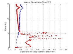 |
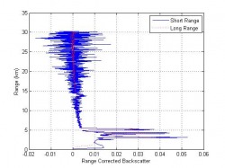
The two graphs above are the Range Corrected Backscatter and Average Depolarization graphs for this data set. Both indicate that something wonky was happening between 3 and 5 kilometers. Both of these graphs are average over time, so they do not show when whatever was happening, but they do both suggest that whatever was happening at that altitude was out of the ordinary. Most of the time, these graphs are relatively vertical, but the data being skewed to the right suggests something else. There is nothing special about this altitude, according to the Depolarization Ratio graph. However, the Range Corrected Backscatter graph shows thick clouds occurring at this altitude. We should keep our eye on these two graphs for future data sets to see if they always respond in this way to thick clouds at mid-lying levels.
The non-colorized Range Corrected Backscatter graph and the Depol Ratio and Range Corrected Backscatter graph both indicate that something happened at 14km and that there was a lot of signal coming from around 2-5km. The 14km can be seen in the top two graphs, and has been explained in the previous paragraph. The signal between 3-5km likely came from different sources. Between 4-5km on the top two graphs, right about 12:00pm GMT, there was some backscatter that was not depolarized. Since that was around the same time that clouds were observed to saturate both the short and long range channels, this backscatter was probably due to the spherical water droplets in low altitude clouds. The signals from 2-4 km were more likely those occuring from 1:00pm GMT until EARL was shut down at 2:20pm GMT. These backscatter signals were not depolarized, and so were likely from spherical particles. Once again, clouds are likely. Since this point in time did not have a cloud cover, the clouds were not thick enough to saturate the channels, as happened at 12:22pm GMT. Therefore, it is also likely that much of the backscatter was due to spherical water droplets in the air itself, due to humidity or the lead-up to a heavy rain. This type of signal and weather should be kept an eye on in the future to see if it repeats itself.
The night is clear, with little Background.
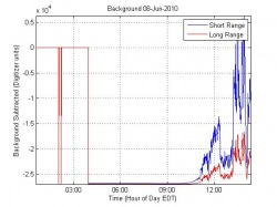
It is interesting for future notice and for projects requiring clear sky data that the background signal during nighttime, as calculated and plotted by the Background graph to the right, is relatively inexistent, especially in comparison to the noise that occurred when the boundary layer started heating up in ernest at about 11:00am GMT. Also, the dip in background noise at about 12:20pm GMT is significant, because that is when the cloud mask was placed on the primary mirror. The noise resumes about at 1:10pm GMT, which is about the same time the cloud mask was removed from the primary mirror. This indubitably says something about the effect of the cloud mask on background noise. The cloud mask effectively cut the background noise in half! While nighttime should be best for observing without background noise, as is obvious from the lack of noise on the early hours of the Background graph, observing without background noise in the boundary layer should be more efficient with a cloud mask. However, this might also be due to the mask limiting the amount of counts of light that the EARL recieves, and therefore skews the data just as much as it clarifies. If a parameter were added to correct for the amount of light that the cloud cover prevents EARL from receiving, then the Background would likely also have a correction that makes reinstalls the amount of background noise that would have been there without the cloud cover.
